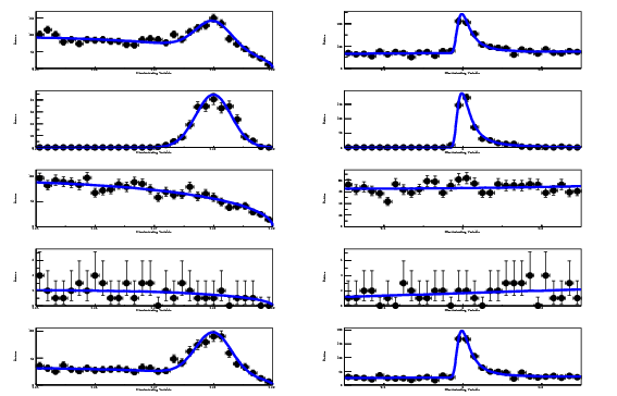
Fig 1: The results of various generated samples obtined (and the PDF projections on the samples) for a two-dimensional signal + background likelihood.
The example rareBdecay.cc is an illustration of how to make a 2D fit model for signal and background. There are two types of background in this model in addition to the signal. A sample of simulated data is generated from the PDF for each of these models, and the data and PDF are plotted at the end of the example. The configuration file for this example is rareBdecay.txt. The model is constructed in the usual way for a simultaneous PDF with
  AFitMaster master("rareBdecay.txt");
  RooAbsPdf * pdf = master.getSimPdf();
then the fit variables are extracted in order to state the process of generating samples of data to plot using
  RooArgSet * compSet = pdf->getComponents();
  RooArgSet * parSet  = pdf->getParameters(compSet);
  cout << "Model Parameter Set:" << endl;
  parSet.Print("v");

  RooRealVar * bMes = (RooRealVar*)parSet->find("bMes");
  RooRealVar * bDeltaE = (RooRealVar*)parSet->find("bDeltaE");

  RooAbsPdf * signalpdf = compSet->find("signal");
  RooAbsPdf * continuumpdf = compSet->find("continuum");
  RooAbsPdf * Bbg0pdf = compSet->find("Bbg0");
Data samples are then simulated using the AFitToy class (See the toy example page):
  cout << "Generating Data" << endl;

  AFitToy toyUtil;
  toyUtil.setPoisson(kFALSE);
  RooDataSet * data    = toyUtil.generateToySample(pdf, RooArgSet(*bMes, *bDeltaE), 2550);
  RooDataSet * sigdata = toyUtil.generateToySample(signalpdf, RooArgSet(*bMes, *bDeltaE), 500);
  RooDataSet * bgdata  = toyUtil.generateToySample(Bbg0pdf, RooArgSet(*bMes, *bDeltaE), 50);
  RooDataSet * cdata   = toyUtil.generateToySample(continuumpdf, RooArgSet(*bMes, *bDeltaE), 2000);
The rest of the example macro concentrates on plotting each of the samples of data
with the associated PDF (all, signal, continuum background, and B background) for
the two fit variables bMes and bDeltaE. This example outputs the plots shown in Figure 1.

Fig 1: The results of various generated samples obtined (and the PDF projections on the
samples) for a two-dimensional signal + background likelihood.
The top row of plots are projectections for the whole data set. The second row shows the signal distributions. The third and fourth rows are continuum and B background, respectively. The last row corresponds to projections made in order to enhance the signal by cutting on the variable integrated over in order to make the plot (i.e. cut on bDeltaE to plot bMes etc.).
This page is maintained by Adrian Bevan.